Lifetime- and Economic Efficiency Simulation of LED Luminaires in Dymola/Modelica

LED lighting is about to replace all conventional lighting technologies, e.g. incandescent lamps or fluorescent lamps. This revolution of the lighting industry was triggered by the rapid development of LEDs due to their luminous efficacy, lifetime and costs.

The lifetime of an LED system is specified by the manufacturer. In general, this value is based on the LM-80 report [I] and is calculated using the TM-21 method [II]. The result is transferred to the manufacturer's datasheet. Unfortunately, this value is solely valid for one specific application. Moreover, this application is not regulated by law and can be defined by the manufacturer. A common application is, for example, to use an ambient temperature of 25°C, a continuous full load operation and a specified maximum allowed decline of luminous flux by 30%. In further consequence the specified lifetime will be used to calculate the economic efficiency of a lighting installation to compare the costs and benefits of the investment.

However, this practice raises a number of delicate questions, particularly with regard to comparability and accuracy:
• How to compare two lighting products with different lifetime information.
• What is the lifetime if a dynamic operating cycle is used?
• What is the lifetime if a dynamic ambient temperature is given?

To answer these questions sufficiently accurate, an LED model has to meet the following requirements: The electric- and thermal behavior has to be described properly. Ageing, i.e. the decline of luminous flux for different operating cycles, e.g. full load, office or industry has to be modeled. Finally, by utilizing the results from the ageing model the economic efficiency has to be calculated.

In the following paragraphs, the current situation and then a new modeling approach are briefly described and the models of the Modelica library DynaLed are introduced. After explaining how a simulation has to be set-up, an application example is shown and the simulation results are discussed. At the end the most important results will be summarized.

Modelling Approach

The basic concept of the modelling approach is shown in figure 1

Figure 1: Simulation approach

Basically, the simulation approach can be separated into two main parts. The first part describes the inputs for the simulation model. Thereby, it is important that all required inputs can be provided easily by the user.

These inputs are:

• Datasheet of the LED: has to be provided by the LED-chip manufacturer and includes information about the maximum ratings and the characteristic values.
• LM-80 Report of the LED: has to be provided by the LED-chip manufacturer and includes measurement data of the lumen maintenance and the chromaticity for a minimum of 6000 hours.
• Operating Cycle: must be provided by the user and gives information about the operating time and operating mode of the LED in each time step.
• Other Information: must be specified by the user and provides information about the environment, the system and the costs.

The second part of the simulation approach describes the implementation of the models in Modelica.

This part consists of the following models:

• Electrical LED model: parametrizable with the information from the LED datasheet.
• Thermal model: parametrizable with the information from the LED datasheet and user information about the heatsink.
• Ageing model: parametrizable with the LM-80 Report and calculated with the output from the electrical and thermal model.
• Economic efficiency model: parametrizable with 'other information' and calculated with the output from the ageing model.

Both parts present their own challenge concerning the implementation. On the one hand the inputs should be modelled in a user-friendly way and on the other hand the simulation environment should have a high degree of flexibility with regard to different LED systems. By contrast the difficulty of the implementation of the test environment is to achieve a balance between the computation time, complexity and accuracy of each part of the simulation environment.

In addition, all implemented blocks should serve as a basic library for dynamic lifetime simulations and profitability assessments of LED systems in the concept stage of the development as well as for products which are already on the market.

Simulation Library

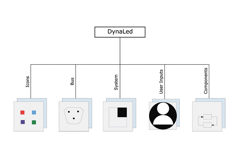
The structure of the DynaLed library for lifetime- and economic efficiency simulation of LED systems is depicted in figure 2.

A short description of each package is given in the list below:

• Icons: Includes all icons of the models provided within the library
• Bus: Contains all variables of interest. Adapters are used to write signals on the bus and read signals from the bus
• System: Consists of the template of the entire system and the data record for the model parameterization
• User Inputs: Includes a model for the operating cycle and a model for 'other information' e.g. the ambient temperature
• Components: This package includes the models and its accompanying sub models for the LED, the heatsink, the lifetime- and economic efficiency calculation

Figure 2: Package structure of the library

The implementation of the entire system is similar to the simulation approach and is illustrated in figure 3. It consists of five main parts: the user inputs, the luminaire model, the ageing model, the maximum ratings and the economic efficiency model. Additionally, the luminaire model is split into an LED model and a heatsink model. This design is chosen because each model can be replaced individually, leading to a high degree of flexibility.

Figure 3: Top level of the entire model

For the data transmission between the different modules a bus is used. To clearly represent which signal is written to the bus and which is read from the bus, adapters are designed. Therefore, for every signal on the bus a writing adapter and a reading adapter is created.

User Inputs and Data Supply

The required user inputs are separated by the source of origin, i.e. datasheet, LM-80 report, operating cycle and 'other information'. Furthermore, the entire data supply of the models in the DynaLed library is done via the data record, shown in the middle of figure 3. A record is a collection of the model parameters. To parametrize the entire system model shown in figure 3 the record is instantiated and the parameters are propagated to each model.

Luminaire Model

The luminaire model is separated into an electric model and a thermal model.

Electric Model

An LED is a special kind of diode. The difference to a regular diode is that the LED model is a combination of an electric power model, a photometrical power model and a thermal power model. The schematic signal flows are shown in figure 4.

Figure 4: Signal flow of the LED model

The top level of the LED model is implemented according to figure 4 and is shown in figure 5.

Figure 5: Top level of the LED model

Figure 6 shows the entire electrical power model of the LED. On the top, the electric circuit is modelled consisting of the ballast and an LED. On the bottom, the power consumption calculation of the system with the unit Ws is implemented. Since the electric circuit is solely modelled for a single LED, the measured power consumption is scaled with the number of LEDs in the luminaire. The output of the model is the forward current and the power of the electric circuit.

Figure 6: Implementation of the electrical power model

The ballast is required for the power supply of the LED. The ballast is modelled using an ideal current source which is driven by the product of the normalized operating cycle and the nominal forward current of the LED. Therefore, the output current is adjusted depending on the operating cycle.

Additionally, the following assumptions for the model of the ballast were made:

• It is an ideal ballast, i.e. its efficiency is 100%
• The lumen output of the LED is linearly depending on the current input

The electrical properties of an LED are equal to the electrical properties of a diode, i.e. to simulate an LED the diode model will be used. There are mainly three different techniques to model a diode: ideal modelling, physical modelling and behavioral modelling. The ideal model has the disadvantage of precision; drawbacks of the physical model are the parametrization and the simulation performance. Therefore, the most suitable modelling technique is behavioral modelling, because it can be parametrized with parameters and characteristic curves from the datasheet and the results are usually accurate enough to get an understanding of the real behavior of the system.

The LED model is shown in figure 7. The current sensor measures the input current of the LED, which is the input for the table containing the forward characteristic curve of the LED specified in the datasheet. The output of the table is the current depending forward voltage drop. Additionally, the forward voltage depends on the junction temperature. This dependency can be found in the datasheet as well. To take this into account the percentage voltage drop depending on the junction temperature at a reference forward current is multiplied with the forward voltage, refer to equation 1. This voltage is the input to the signal controlled voltage source.

   EQ1

Figure 7: Implementation of the LED

The photometric power model is also a static behavioral model, see figure 8. The forward current of the LED is the input for the table containing the relative luminous flux characteristic curve of the LED which is specified in the datasheet. The output of the table is the current depending relative luminous flux. Additionally, the luminous flux depends on the junction temperature. To take this into account the relative luminous flux drop depending on the junction temperature is multiplied with the relative luminous flux. To get the absolute value of the luminous flux the relative luminous flux depending on the junction temperature and the forward current is multiplied with the reference luminous flux value.

The next step is to calculate the luminous efficacy of the LED. Therefore, the ratio of luminous flux and electrical power is computed. Based on this and the maximum possible luminous efficacy [III] depending on the spectral emission the photometric output power is calculated which represents the output of the model.

Figure 8: Implementation of the photometric power model

According to the principle of conservation of energy the thermal power is the subtraction of the photometric power from the electric power. This calculation is done in the thermal power model shown in figure 5.

Thermal Model

The thermal model is implemented as a Cauer-network. The losses from the thermal power model of the LED are the source of heat flow entering at the junction interface. The heat is transported through the thermal resistance from the junction to the solder point to the heatsink and to the atmosphere. The temperature profile of the ambient temperature is specified in the ‘other information’ model shown in figure 3.

Additionally, the dynamics of the thermal model are implemented using the heat capacitors of the different elements. All the heat capacitors have to be initialized with the ambient temperature because it is assumed that the system has been long enough in its ambient state that it has adopted this temperature level.

The implementation is shown in figure 9. The output of the thermal model is the solder point temperature of the LED.

The values for the thermal resistances and the heat capacitors can be taken from the corresponding datasheets are calculated with the geometrical boundary conditions and material or have to be evaluated via temperature measurements.

Figure 9: Implementation of the thermal model

Ageing Model

The ageing and therefore the lifetime of an LED-system depends on a multitude of influential factors.

The most important factors are listed below:

• Temperature: the heat which is produced from losses of the LED has negative effects on several LED parameters, e.g. the lifetime, the luminous flux, etc.
• Current: each LED is driven with a certain electrical current. The amplitude of this current has a direct effect on its lifetime. The lower the current, the lower the heat generation and the higher the lifetime.
• Radiation and light: the light which is emitted by the LED has an ageing effect for example on the housing or the reflector.
• Mechanical forces: the reason for applying a mechanical force can be a faulty assembly, high temperature fluctuations, etc. The effect is a premature failure of the LED.
• Humidity: can lead to corrosion of metal parts inside the LED-module and therefore to a premature failure.
• Chemicals: chemical substances, like high sulfur dioxide content of the air, have a negative effect on the lifetime of the LED [16].

For the ageing model the influential factors temperature and current are the only being considered, because in comparison radiation and light have a relatively small impact on the lifetime of an LED. The other three factors are influenced by the end user and can therefore not be considered in a meaningful way.

Figure 10: The ageing model is based on the TM-21 calculation method which is based on the exponential decay, see equation 2

   EQ2

Where t is the operating time in hours, Φ the averaged normalized luminous flux output, B the projected initial constant derived by a least squares curve-fit and α, the decay rate constant derived by a least squares curve-fit as well.

After reformulating equation 2 to equation 3, the time to reach a specific L_x value [IV] can be calculated. [2]

   EQ3

Equation 3 is implemented in the ageing model depicted in figure 10. The inputs are on the one hand the forward current from the electric model and on the other hand the solder point temperature from the thermal model. The actual values for the start value B and the decay constant α are stored in a table and are dependent on the inputs.

The result of equation 3 is the lifetime of the system depending on the forward current of the LED, the solder point temperature and the specified L value. Due to the fact that the forward current and solder point temperature changes dynamically the percentage ageing is integrated over time. Therefore, the result of the ageing model is the percentage ageing of the system after the reviewed simulation period.

Maximum Ratings

The task of this model, shown in figure 3, is to monitor the maximum ratings. For a reliable long-term operation of the LED it is important that these values are not exceeded.

The following values are monitored:

• Operating temperature
• Junction temperature
• Solder point temperature
• Forward current

If one of these values exceeds the permitted range the simulation is terminated.

Economic Efficiency Model

For a meaningful simulation of the economic efficiency the following aspects of a lighting system have to be addressed:

• Investment
• Energy procurement costs
• Lighting hours
• Plant lifespan
• Nominal lifetime of the lighting system
• Installed power including all auxiliary units, e.g. ballasts
• Maintenance costs

The economic efficiency model evaluates the total investment I_tot of a lighting system over a specified period of time. The total investment can be computed with equation 4. It is the sum of the initial investment I_I for the luminaires including the ballast and the installation, the energy costs I_E for the review period and the replacement costs I_R for the luminaires.

   EQ4

The initial investment I_I consists of the costs for a luminaire I_L including the ballast and the installation costs per luminaire I_In. This value is multiplied by the number of installed devices N, see equation 5.

    EQ5

The energy costs I_E are the product of the average energy consumption E_a of the luminaire including the efficiency η of the ballast, the number of installed devices N, the electricity costs I_kWh and the time period under review t. The calculation is done with equation 6.

   EQ6

If a luminaire comes to the end of its lifetime it has to be replaced, i.e. a new luminaire has to be installed. Therefore, each replacement means that an investment in the amount of I_I has to be arranged. The number of replacements is dependent on the period under review t and the lifetime of the system t_end. The replacement costs I_R can be computed with equation 7.

   EQ7

Running a Simulation

To keep the application of the DynaLed library as simple as possible two functions have been created: One for the lifetime- the other for the economic efficiency calculation.

The function for the lifetime calculation simulates the entire system model from figure 3 for a period of 24 hours, i.e. the stop time of the simulation is 86400 seconds. Depending on the behavior of the system in this period all values are extrapolated. For example, in order to compute the entire lifetime of the LED, the output of the ageing model, i.e. the ageing after 24 hours, is extrapolated.

This can be done because the model underlies following assumptions:

• The operating cycles are repeated every 24 hours.
• The ageing model does not consider the calendrical ageing, i.e. the ageing is solely depending on the solder point temperature and the forward current of the LED.

After executing the function for lifetime calculation the results are used to parametrize the economic efficiency model. Afterwards, the function for economic efficiency calculation is called.

The output contains the following results:

• Total investment for the reviewed lifespan
• Initial investment for the luminaires and the installation cost
• Energy costs for the reviewed lifespan
• Number of required replacements of the luminaires

Application Example

An application example, which is available on the market, is used to show the function of the DynaLed library in a real system. The LED System is simulated utilizing the developed Modelica library and the economic efficiency of different operating cycles are compared.

System

The simulated luminaire is an LED louvre luminaire (Article Code: 29001077 - for more information refer to [17]). The light sources of the luminaire are 104 pieces DURIS E5 LED from Osram (Type: GW JDSRS1.EC-FUGQ-5L7N-L1N2). The power supply of the LED is a constant current ballast.

The following three different types are available:

• Ballast DALI dimmable
• Ballast DALI dimmable
• Ballast 1-10V dimmable

The used ballast type depends on the application and in further consequence on the operating cycle.

Results

The results are separated into lifetime calculation results and economic efficiency calculation results.

Lifetime Calculation Results

The lifetime of the system depends on the one hand on the forward current and on the other hand on the solder point temperature of the LED. Therefore, the lifetime of the system varies, depending on the used operating cycle (OC). For the simulation seven different operating cycles are considered. Five of them are appointed to different areas of application and are translated from the human centric lighting curves from [18]. Additionally, a full load operating cycle and a constant light output are added.

The following different operating cycles are used for the simulation:

• Full load (FL)
• Constant light output (CO)
• Education (ED)
• Health and care (HC)
• Office (OF)
• Shop and retail (SR)
• Industry (IN)

Additionally, the average power of the system also depends on the operating cycle.

The results of the different simulation runs are listed in table 1.

Operating Cycle	Lifetime [h]	Power [W/Luminaire]
FL	45 564	40.13
CO	56 518	35.83
ED	155 119	19.83
HC	92 475	23.09
OF	109 362	22.84
SR	138 086	14.50
IN	73 921	31.73

Table 1: Results of the lifetime simulation

It must be noted that according to the limits of the TM-21 calculation method, only the lifetime of the full load and the constant light output operating cycle are within the boundaries. To verify the lifetime of all operating cycles an LM-80 report is required with a testing period of 26000 hours. Nevertheless, the simulation shows that the lifetime of the system is strongly dependent on the used operating cycle.

For further consideration the values from table 1 are not adjusted and are directly used to parametrize the economic efficiency calculation.

Economic Efficiency Calculation Results

For the economic efficiency calculation a simulation period of 100000 hours was assumed. Furthermore, the purchase price of a luminaire including the ballast, the installation costs and the energy costs are required. These costs depend on a variety of different factors.

Some of them are listed below:

• Purchase price of a luminaire including the ballast
  • Depends on the used ballast. The non-dimmable ballast is cheaper than the ballast with constant light output. Additionally, the ballast with constant light output is cheaper than the DALI dimmable ballast. The result is that depending on the operating cycle a suitable driver needs to be selected which has an influence on the price.
  • Depends on the discount level of the customer.
• Installation costs
  • Depends on the ballast used. The luminaire with the DALI dimmable ballast results in additional installation effort, e.g. more wires, sensors, programming, etc.
  • Depends on the hourly labor costs of the installer.
• Energy costs
  • Depends on the contract with the energy provider.
  • Depends on the cost increase over the period under review.

According to the multitude of influencing factors there are no generally valid values for the required parameters. The used parameters are listed in table 2.

Operating Cycle	Luminaire [€/Luminaire]	Installation [€/Luminaire]	Energy [€/KWh]
FL	120	25	0.15
CO	170	25	0.15
ED	200	50	0.15
HC	200	50	0.15
OF	200	50	0.15
SR	200	50	0.15
IN	200	50	0.15

Table 2: Required parameters for this example

The results of the economic efficiency calculation are the total investment I_tot, the initial investment I_I, the energy costs I_E and the number of replacements N_R, see table 3.

Operating Cycle	Itot [€]	II [€]	IE [€]	NR
FL	27 594	3 625	16 719	2
CO	24 679	4 875	15 929	1
ED	14 416	6 250	8 166	0
HC	22 125	6 250	9 625	1
OF	15 750	6 250	9 500	0
SR	14 416	6 250	8 166	0
IN	25 708	6 250	13 208	1

Table 3: Results of the economic efficiency calculation

Interpretation

The influence of different operating cycles on the lifetime of an LED luminaire and in further consequence for the total costs are depicted in table 1 and table 3.

One illustration is the following: the lifetime of the luminaire increases by a factor 3.4 if the education operating cycle is used instead of the full load one. The full load operating cycle has the advantage of a 42 % lower initial cost, because a non-dimmable driver can be used and no additional installation effort is required, the disadvantage is an increase of the total costs by 91 % if an economic efficiency calculation for a review time period of 100000 hours is done.

Conclusion

The developed library is a convenient tool for manufacturers for lifetime- and economic efficiency simulations of LED systems. The implementation provides a simple and time saving method for any kind of adaptions. It allows the user to simulate and compare different kinds of luminaires with the same library. Furthermore, the handling of the library and the data supply is implemented in a user-friendly fashion.

Notes:

[I]          A record of the lumen maintenance, the chromaticity and the catastrophic failures of LEDs. This test will be done at three LED case temperatures (55°C, 85°C and one selected by the manufacturer). The minimum testing period is 6000 hours, whereby the data collection has to be done every 1000 hours. The LM-80 report is provided by every renowned manufacturer. For further information refer to [1].

[II]         The TM-21 specifies how to extrapolate the LM-80 lumen maintenance data to times beyond the LM-80 test time [2]. The disadvantage is that this model is only valid for steady-state applications.

[III]        The calculation of the maximum luminous efficacy depending on the spectral emission is based on [15]. For the calculation the spectral emission of the LED and the photopic sensitivity curve of the human eye is required.

[IV]        The L_x value describes the reduction in luminous flux. Whereby, x provides the information about the minimum level of acceptable lumen output in percent.

[V]         For a sample size of 20 units, the maximum projection is 6 times the test duration of the LM-80 report. [1]

References:

[1]         E. Richman. The elusive ‘life’ of leds: How tm-21 contributes to the solution. LEDs Magazine, 6, 2011.

[2]         M. Scholdt. Temperaturbasierte Methoden zur Bestimmung der Lebensdauer und Stabilisierung von LEDs im System. 2013.

[3]         M. Otter, H. Elmqvist, and S. E. Mattsson. Hybrid Modeling in Modelica based on the Synchronous Data Flow Principle. 1999.

[4]         S. O. Kasap. The pn Junction: The Shockley Model. 2001.

[5]         A. Wintricht. Verhaltensmodellierung von Leistungshalbleit- ern für den rechnergestützten Entwurf leistungselektronischer Schaltungen. 1996.

[6]         P. Denz, T. Schmitt, and M. Andres. Behavioral Modeling of Power Semiconductors in Modelica. 2014.

[7]         A. Courtay. MAST power diode and thyristor models including automatic parameter extraction. 1995.

[8]         D. Madur, N. Ghatte, V. Pereira, and T. Surwadkar. Modelling light emitting diode using spice. 2013.

[9]         MathWorks. Documentation: Light-Emitting Diode. www.mathworks.com, Accessed 2017.

[10]       Cree. Thermal Management of Cree® XLamp® LEDs. www.cree.com, Accessed 2017.

[11]       Vossloh-Schwabe. Thermal Design of LED Luminaires. www.vs-lighting-solutions.com, Accessed 2017.

[12]       C. C. Karl. Einfluss von Wasserstoff auf das Alterungsverhalten von InGaAlP Leuchtdioden. 2014.

[13]       LED Blog. Stromrechner für LED Lampen. www.leds-blog.de, Accessed 2017.

[14]       Lichtspur. Wirtschaftlichkeitrechner. www.light-trail.com, Accessed 2017.

[15]       W. Thomas and Jr. Murphy. Maximum Spectral Luminous Efficacy of White Light. 2013.

[16]       Osram. Zuverlässigkeit und Lebensdauer von LEDs. 2008.

[17]       LEDON Lamp Gmbh. Impressum. www.ledon-lamp.com, Accessed 2017.

[18]       Trilux. HCL-Kurven. www.trilux.com, Accessed 2017.