Optimization of Freeform Optics Using T-Splines in LED Illumination Design

The design of free-form optics relies heavily on one of the methods: tailoring based on point source assumption [3], SMS design [4] and source target maps based on equal flux grids [5] to create an initial optical surface. As these mathematical methods are not guaranteed to provide accurate results for extended LED sources and as well do not provide generalized solutions, the optical designer still relies on any optimization tool to improve the results. The improvement of speed in raytracing algorithms as well as sophisticated intelligent optimization algorithms make an optimization approach more widely usable. But the drawback of optimization in freeform surfaces is mainly because of its complicated mathematical representation and the presence of many parameters. These parameters are not directly related to the optical performance hence making the optimization a long process to meet the needed lighting requirements.

Wendel et.al proposed a method called optimization using freeform deformation (OFFD) to overcome this difficulty by placing the optical surface in a grid and deform the enclosed lattice rather than acting directly on them [1]. This method uses NURBS to represent the optical surface and their results show that with fewer optimization variables, they could attain global deformation very well, and this makes manufacturing easier. But there are certain cases which require a sharp gradient in the light distribution or a path of the light ray has to be changed significantly. In such cases, a slight local deformation brings significant improvement. But with the current OFFD, it is not possible because of the underlying surface representation. An alternate surface representation called T-splines could overcome this drawback [2]. Bailey et.al has shown the potentiality of T-splines and its application in optical surfaces [6]. But this has neither been applied in any optimization routine so far nor its optical performance analyzed and compared against NURBS.

So this work takes this problem into account and provides an alternate way to solve this problem. Section 2 covers the OFFD technique. The mathematical surface representation of optical surfaces is covered in section 3. The implementation results of T-splines and comparison results are shown in section 4 followed by the conclusion in Section 5.

Optimization Using OFFD

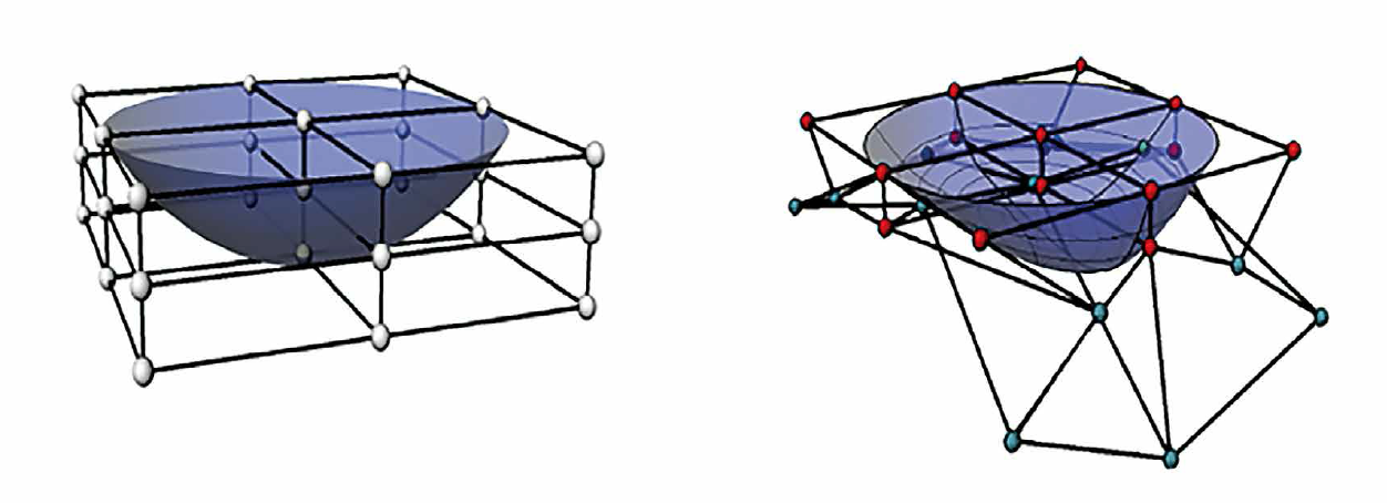
OFFD methods employ freeform deformation (FFD) technique proposed by Sederberg [7] coupled with an optimization routine. The relationship between the grid and the optical surface is well established using the FFD algorithms [7]. Figure 1 shows the grid with an optical surface before and after deformations. For conciseness, only an overview of the OFFD method is explained.

Figure 1: A 3x3 OFFD grid enclosing and optical surface before (left) and after (right) deformation

The algorithm begins by selecting an input surface whose optical performance has to be improved, which is usually far from the target. By this method, the optical surface is enclosed inside the grid containing 27 grid control points and the user could select any combination out of them. This is provided as variables to the optimization algorithm. The optimization algorithm has a wide search space for the selected combination of grid points and provides shifts along the three dimensions to the enclosed grid. As the enclosed grid undergoes a change, it changes the optical surface inside too. The deformed surface is then evaluated photometric and the optimization algorithms take decisions about the shift of its optimization variables based on this result. This algorithm continues again and again until the target lighting requirements are met. The workflow is explained using the flowchart in figure 2.

Figure 2: Workflow of the optimization of freeform deformation (OFFD)

The most important step in this routine is the definition of Figure of Merit for the deformed optical surface as the entire optimization is based on this single value referred as Q. In this paper, we use two different merit functions.

Deviation merit function Qdev which corresponds the deviation of the current simulated distribution and the desired distribution and is expressed as

G is the area that one is interested in, Eideal(x) is the desired illuminance distribution target and E(x) is the current light distribution.

Flux based merit function Qflux corresponds to maximizing the flux in the required target area which is quantified as ratio of flux in the target (Φt) and available flux collected by optics Φc.

Mathematical Representation of Optical Surfaces

NURBS
NURBS techniques are so mature that they are used in computer-aided graphics systems as well as ray tracers. Due to its flexibility, the surfaces can be easily manipulated or modified by changing the control points or its weights during the optimization routine. NURBS surface is the parametric tensor product surface and is defined as:

where Pij is (n+1) x (m+1) rectangular array of control points, wi,j are the weights, Nip(u) and Njq(v) are basis functions of degree p and q in u and v directions, respectively associated with the knot vectors.

where r=p+n+1 and s=m+q+1 hold. When a control point has to be added in NURBS, it is done using the knot insertion method. Addition of a single knot requires adding an entire column or row of control points. Knot removal is also not possible with NURBS without a change in the shape of the geometry. This local refinement is mainly limited in NURBS because of its tensor product construction as shown in EQ 3. As seen in figure 3, the NURBS surface is repeated horizontally column by column and vertically row by row. In order to satisfy this balance, if one adds a new control point, the entire column or row of control points gets simultaneously added.

Figure 3: An example showing the initial 5x5 NURBS patch (left), how the modification causes addition of control points along rows and columns when done with NURBS (middle) and in T-splines (right)

T-splines
The drawbacks imposed by NURBS can be solved by an alternate mathematical representation of the freeform surfaces called as T-splines. T-splines generalizes B-splines to assign particular row and column parameters to the specific control points by adding T-junction to B-splines which is seen relevant in figure 3. This makes T-splines a more advanced technique in local deformation without adding unwanted control points. A T-spline is a tensor product B-spline which is point based rather than grid based. The control grid is called T-mesh and definition of a T-spline surface is given by

where Pi are control points. Ni(u,v) are basis functions, given by

The basic functions Nui(u) and Nvi(v) are respectively associated with knot vectors

When one inserts a new control point or a knot, the interval between the other control points has to be refined without any change in its shape. This is done as the refinement of two univariate basis functions Nui(u) and Nvi(v) separately by fulfilling EQ 6. This property of local refinement without increase in the number of control points as well no change in the shape of the geometry makes T-splines naturally a good choice to implement in the OFFD and attain local deformation.

Figure 4: Initial optical surfaces segmented into 6 sections (left) and the OFFD grid with numbered control vertices (right) ready for local deformation

Application of T-Splines in OFFD

The last section covered the theoretical background of T-splines and advantages of using it in the local deformation. This section presents the application of T-splines in the optimization routine of the freeform deformation system explained briefly in section 2. For our example, we used the same optical design task of designing a street light lens used in [1]. Cree XPG2 LED with 100 lumens is used as a light source and the initial surface before optimization is as shown in figure 4. To evaluate the photometric performance, the merit functions expressed in equations 1 and 2 are applied.

To begin the T-spline implementation in OFFD, one has to add more control points in the needed regions and the shape of surface stays unchanged. More local deformation is achieved in the regions of the area where more and denser control points gather. A study was then conducted to find which part of the lens is influenced more by the deformation process and if the sensitive local deformation on this part leads to a better result.

The whole optical surface is separated into six sections, as shown in figure 4. This step is based on an intuitive assumption. The symmetry in the y-direction is due to the fact that the target street and the lamp stay in the middle of y-direction (Figure 5). For a straightforward comparison, the grid points [1, 3, 13 15] are chosen. More control points are added in each segment from 1 to 6. In the end, six new optical surfaces are generated. The only difference between these generated new T-spline surfaces and the initial one is the difference in the number of control points. The shape of the optics maintains the same without any variation as expected. These optical surfaces are taken as initial surfaces one after the other for the OFFD and are evaluated using both the described merit functions. The preliminary results showed that more impact on the light distribution is seen when more control points are added to the segment 5. So this optical surface with more control points at segment 5 and less at the remaining sections is taken as an initial system for optimization and for comparison against NURBS. This result is then compared with the NURBS-based OFFD and the results are discussed in the coming section.

Figure 5: Schematic view of the street lighting setup with 10 m pole spacing, 6 m pole height, 1 m distance away from the road. The yellow rectangle shows the area to be illuminated [1]

Performance of the initial system
The optical performance of the initial surface is shown in figure 6 with only 15% of total flux inside the target and the shape of the distribution is far away from the needed rectangular distribution which is marked as white.

Figure 6: Illuminance distribution of the target street area (white rectangular frame) for the initial surface shown on the left

Figure 7: Illuminance distribution of the streetlight lens with more control points on the fifth section (a) using T-splines using deviation merit function (b) flux based merit function (c) NURBS using deviation based and (d) flux based merit functions

Comparison between NURBS and T-splines
The two important photometric measures for comparing NURBS and T-splines used in analyzing the street lighting lens are total luminous flux in the target and uniform illumination distributed well across the target. NURBS and T-splines perform at the same level for total luminous flux in the target which is found to be as 55% as illustrated in figure 7b and 7d yielding 40% improvement (Δη). But T-splines outperform in shaping the target distribution as required which is validated in the simulation results in figure 7a. The illuminance distribution using T-splines is more uniformly distributed than those with NURBS as shown in figure 7b. The deformed optical surface using NURBS and T-splines is shown in figure 8. The slight difference is seen in the T-splines near the edges which is marked as segment 5 in figure 4. This is the segment where more control points have been added prior to deformation and performed better compared to others.

Figure 8: Deformed optical surface using OFFD NURBS based (left), T-splines based (middle) and the false color representation of the change in shape between NURBS and T-splines (right)

If the same results need to be attained using NURBS, the control points in the grid are more sensitive to the user’s choice. When accurately chosen, one could attain these results but at the expense of the optimization’s runtime which is so long - almost twice the time needed using T-splines. The most advantage in using T-splines is that when the user knows the section of the optical surface to be locally deformed he can be least bothered about the selection of the control points in the grid.

Conclusion

This work highlighted the use of T-splines for obtaining a local deformation of the optical surfaces by implementing it in the optimization routine for the first time. The results show that with T-splines one could attain more uniform light distribution as against NURBS. The sensitivity of the FFD grid points is reduced when T-splines is used. This is very important for intelligent optimization systems. As T-splines is a more advanced surface representation, it is still not yet mature. The CAD techniques and ray tracers have not grown to an extent to import and work directly with the T-splines file format. So at the time of this paper, one needs to still rely on back and forth conversion of T-splines to NURBS to perform raytracing. Another limiting factor, but not huge, is that the control points have to be added more precisely where it is needed. In future, if intelligent optimization systems could be able to predict the segments of the optical surface automatically, then the machine could add them completely and carry optimization routine.

References:
[1] Wendel, Simon, Julian, Kurz and Cornelius Neumann. “Optimizing non imaging freeform optics using freeform deformation”. Proc. Of SPIE, Vol.8558.2012

[2] Scott, M.A., et al. “Local refinement of analysis-suitable T-splines”. Computer Methods in Applied Mechanics and Engineering 213 (2012): 206-222

[3] Ries, H. and Muschaweck, J. “Tailored freeform optical surfaces.” JOSA A 19.3 (2002): 590-595.

[4] Beni, Pablo, et al. “Simultaneous multiple surface optical design method in three dimensions.” Optical Engineering 43.7 (2004): 1489-1502.

[5] Fournier, Florian R., William J. Cassarly and Jannick P. Roland. “Fast freeform reflector generation using source-target maps.” Optics Express 18.5 (2010): 5295-5304

[6] Bailey, Edward and Sebastien Carayon. “Beyond NURBS: enhancement of local refinement through T-splines.” Optical Engineering + Applications. International Society for optics and photonics, 2007

[7] Sederberg, Thomas and Scott R. Parry. “Freeform deformation of solid geometric models.” ACM SIGGRAPH computer graphics 20.4 (1986): 151-160