Practical Estimation of Measurement Times in Goniospectroradiometry and Goniophotometry
The angle-dependent characterization of LED modules and lights often raises the question about typical measuring times. In particular, the comparison of spectrometer-based systems with photometer-based systems is of considerable interest here. Dr. Günther Leschhorn, product manager for spectroradiometers and SSL measurement equipment from Instrument Systems GmbH, considers different measurement set-ups in a study and makes recommendations for various application cases.

Two typical SSL-sources with different spatial radiation characteristics and different total luminous flux values are investigated in this study. A goniometer is used in a turning-luminaire and a turning-detector type setup for goniospectroradiometric and goniophotometric measurements on the samples. The study puts a particular emphasis on the required measuring times for the different configurations and validates the data according to the quality of the measurement. The results are used to give some practical guidance on how to choose the measurement setup with respect to detector, resolution, size of the sample and compliance with corresponding standards regulations in the daily laboratory routine.
Introduction
When performing angular-resolved measurements on Solid-State-Lighting (SSL) products, one question is most typical: What is the measurement time I have to consider? The interest lies, in particular, in the different time scales one has to take into account when deciding between spectroradiometer-based and photometer-based systems. Typically, goniospectroradiometry is slower but allows all important performance characteristics such as luminous intensity distribution curves, luminous flux, color coordinates and even color rendering index to be measured with maximum precision. In goniophotometry on the other hand, fast photometers are used which typically reduce the measurement time. Goniophotometry is faster compared to goniospectroradiometry but is restricted to purely photometric quantities.
In most cases, the application defines the need for one detector type or the other. Nevertheless, saving valuable measurement time in the daily laboratory routine is important for most of the users. A photometer as, for example, an add-on to a goniospectroradiometric system has the potential to reduce the overall measuring time significantly. An estimation of the measurement time is therefore valuable information that helps in this decision process.
The time scales of the measurement depend on numerous factors, like spatial radiation characteristics (and with that resolution), number of performed C-planes, applied standard regulations, type of goniometer and size of the sample - just to mention a few. In this study, two showcase SSL-sources are evaluated. These two specimens differ in their spatial radiation characteristics and are measured with different detectors in different measurement geometries. With this data, it is possible to estimate the typical measuring time, the associated errors and to give a few rules of thumb that are of help for the user when it comes to questions concerning measuring times.
Experimental Setup
All measurements are performed with the LGS 1000, the largest goniometer by Instrument Systems. The goniometer is based on the C,γ coordinate system (CIE 121-1996) and accommodates samples up to a diameter of 2 m and a maximum weight of 50 kg. It can be operated with a photometer as a conventional goniophotometer or with a spectrometer as a versatile goniospectroradiometer. For the measurements an array spectrometer (comprising a CAS 140CT with an optical probe) and a photometer is used. The device under test is stabilized according to the procedures described in IES LM-79-08 and EN13032-4. Measurements are performed in a completely dark room featuring matt black walls, floor and ceiling to eliminate undesired stray light.
For the measurements, two different configurations of the goniometer are used, which will be described in the following paragraphs.
Turning-luminaire setup
The standard configuration is a so-called turning-luminaire goniometer conforming to the C,γ coordinate system with a horizontal optical axis. During the measurement, the luminaire is rotated in the horizontal C-axis and the vertical γ-axis. An optical probe for use with the spectroradiometer or alternatively a photometer head is mounted on a tripod stand and aligned with the horizontal optical axis of the test specimen. A baffle-tube to minimize stray light is mounted in front of the detector. The stand accommodating the detector is set up at a distance where the sample can be considered as an approximated point light source (photometric distance) to maintain the far-field condition for luminous intensity measurements. Figure 1 shows the setup of the goniometer in the turning luminaire configuration.
 Figure 1: The goniometer in standard turning-luminaire configuration (left) and detector with stray light tube on stand (right)
The goniometer provides the possibility to adjust the angular speed of both axes. The faster C-axis can be rotated with 16 selectable speeds ranging from 3.1°/s to a maximum speed of 50°/s. The speed of the γ-axis can be selected from 1.8°/s to 30°/s respectively.
Furthermore, the goniometer can be operated in two different measurement modes, the start/stop and the continuous mode.
A sequence measured with start/stop functionality means that each pair of angles to be measured will be approached by the goniometer with the selected speed of the corresponding axis. Once the goniometer has come to a full stop and the angles are reached correctly, the measurement will be triggered. This procedure continues with all angle pairs defined in the resolution requested by the operator. Due to time-consuming acceleration and brake phases, this mode is slow and commonly used with spectroradiometric measurements where longer integration times are needed.
On the other hand, for a continuous sequence a photometer is used. In this mode, the goniometer has only one acceleration and one brake phase and moves with a continuous velocity through the defined angular region. Passing the angles to be measured, the system triggers a measurement “on-the-fly”. This means that the light distribution is measured by the photometer while the goniometer is moving and the digital signal processing of the measurement amplifier ensures optimum adjustment of the integration and filter parameters during the recording. The overall measuring time is significantly reduced compared to the start/stop mode, but yields only purely photometric quantities.
Turning-detector setup
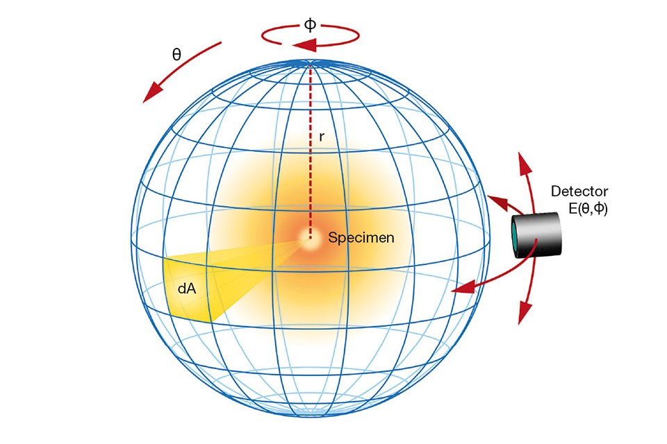
With the help of an additional option, the goniometer transforms into a turning-detector type with vertical optical axis. The setup is illustrated in figure 2. The position of the sample remains unchanged during the measurement and the detector moves around the test specimen on a spherical envelope surface. A spectrometer as well as a photometer can be used as detector. With this option, the sample size that can be used for measurements that require the photometric distance to be maintained is reduced in comparison to the standard configuration. For measurements completely compliant to IES LM-79-08, the diameter is reduced to a maximum of 18 cm. For luminous flux measurements, this restriction does not apply. Figure 2: Turning-detector type goniometer (left) and illustration of operating principle (right)
Due to the transformation in goniometer type, the axes are switched. The γ-axis that is more frequently used in typical measurements of SSL-sources can now reach a maximum velocity of 50°/s and the C-axis can reach a maximum velocity of 30°/s. With this, a further reduction of the overall measurement time can be achieved.
SSL-light sources
To illustrate the dependence of the overall measuring time on the spatial radiation characteristics of the used sample, two different light sources are investigated in this study.
 Figure 3: Relative luminous intensity distribution curves (left side) of the two SSL-sources used in this study. The blue line represents a light source with a rather broad angular distribution and the red line represents a more directional downlight. Absolute luminous intensity distribution of one C-plane in Cartesian representation is given on the right side. The total luminous flux associated with the blue curve is higher than that of the red curve, but the peak luminous intensity is lower
One LED downlight has a rather broad angular distribution with a half angle of approximately 80° (FWHM). A relative luminous intensity distribution curve of this light source is given by the blue line in figure 3 on the left side. The total luminous flux is approximately 670 lm with a CCT of 3500 K and a high CRI value of >95.
With approximately 403 lm, the second source has a lower total luminous flux and different spatial radiation characteristics. With a half angle of approximately 29°, this light source is more directional. A relative luminous intensity distribution curve is given in red in figure 3 on the left for comparison. The Cartesian representation of one C-plane in figure 3 right side, shows the absolute difference in luminous intensity of the two light sources. Although the total luminous flux of the more directional light source is significantly smaller compared to the downlight with broad angular distribution, it has a higher peak luminous intensity by more than a factor of 3. Consequently, the gradient of luminous intensity with angle is much higher.
Estimation of Goniophotometric and Goniospectroradiometric Measuring Times
For the two light sources discussed in the last section, a study of the total measurement time versus resolution with different detectors and settings is performed. The standard turning luminaire configuration is used with a spectrometer as well as a photometer as the detector. The distance between the light source and the detector is set to 3.2 m, in order to maintain the photometric distance.
Spectroradiometric measurements
For the measurements with the spectroradiometer, two different methods to define the integration time are used. The dynamic range in luminous intensity of the light sources over the angular range makes it necessary to adjust the integration time of the spectrometer. Each change in integration time is time consuming, because a dark current measurement is necessary; so changes in integration time should be limited. On the other hand, a high-quality spectroradiometric measurement needs a good signal level. Therefore, a tradeoff has to be found that limits the changes in integration time to a minimum while still maintaining the quality of the measurement. This tradeoff, however, can only be found when the spatial radiation characteristics are already known in the beginning of the measurement which is the case when testing batches of samples of the same kind. In this case, an optimization of the measurement time with a spectroradiometer can be realized. In this section, a worst case scenario is analyzed, assuming that the spatial characteristics are not known.
In order to optimize acquisition, two different approaches are used:
• The integration time of the spectrometer is set to a high signal level near saturation at the peak of the luminous intensity (this peak is assumed to be at the center of the light source). The integration time is fixed and used for all other angles
• The auto-ranging function of the spectrometer is used to adjust the integration time dynamically. Signal levels between 50% and 100% are automatically adjusted. To avoid unnecessary long integration times, the maximum value is set to 3 seconds
 Figure 4: Overall measurement time versus increment for different measurement modes (left) and the corresponding deviations of luminous flux (right) for the sample having a broad angular distribution
With these two approaches, one C-plane in the lower half plane (-90° to 90°) with different increments are measured using the start/stop mode of the goniometer. The total measuring time is recorded. Figures 4 and 5 show the results for the light sources with broad and narrow distribution. The blue (green) line represents a spectrometer with fixed integration time and a spectrometer using its auto-ranging mode, respectively. As expected, the spectrometer in auto-ranging mode generally needs more time to complete the measurement. In general, the curves look very similar. For increments larger than approximately 2° to 3°, the curve evolves into quite a long plateau with increasing increments (equivalent to decreasing resolution). Overall measurement times of a few minutes are typical for this regime. For smaller increments, the measurement time rises steeply. Overall measurement times of tens of minutes up to half an hour must be expected when working in this regime. These data only represent one C-plane. The measured time has to be multiplied by the number of C-planes required for the actual measurement. If an extreme resolution of ≤0.5° is necessary, the overall measuring time might expand to several hours for a typical value of 4 to 5 C-planes.
On the right side of figures 4 and 5, the deviation of the total luminous flux calculated from the measurements is presented. The measurement at 0.2° increment with the spectroradiometer serves as a reference. Due to the rather broad angular distribution light source, no significant deviation can be found up to 8° increment. In figure 4, all measured flux values stay within ±0.2%. The much more directed nature of the distribution of the downlight in figure 5 leads to a different behavior. Up to a resolution of 2° increment, the situation is similar to the situation in figure 4 with a deviation of 0.2% maximum. For larger increment values, the deviation rises and can be clearly above 1%. This will contribute to the user’s measurement uncertainty budget. In praxis, an adaption of the chosen increment to the spatial characteristic of the source can reduce the measurement time as well as the associated component in measurement uncertainty.
Photometric measurements
The measurements described above also have been performed with a photometer as the detector. Therefore, the continuous mode of the goniometer could be used, which allows recording of spatial radiation characteristics “on-the-fly”. The recorded data is plotted in red in figures 4 and 5.
 Figure 5: Overall measurement time versus increment for different measurement modes (left) and the corresponding deviations of luminous flux (right) for the sample having a more directed angular distribution
In contrast to the spectroradiometric measurements, the results of the photometer show no dependency of measurement time on the chosen increment. In fact, all values lie on a constant line at 13 seconds measuring time for both light sources and all increments. This is due to the adaptive adjustment of the digital signal processing of the photometers electronics which ensure a good signal level at all increments. As visualized on the right side of figures 4 and 5, the photometer data show qualitatively the same behavior as the spectroradiometric data for the deviations in luminous flux. Since the measurement with the photometer is so fast, a high resolution measurement with typically 4 to 5 C-planes lasts around one minute.
Summary and practical guide
This section conveys some practical aspects from the results of the last two sections.
If only photometric values like luminous intensity distribution or luminous flux are of interest, it is recommended to use a photometer together with the on-the-fly function of the goniometer. With this type of setup, fast and high resolution measurements can be performed. The photometer should always be used with a low increment like 0.5° or even 0.2°. The measurement time is not affected by the choice of resolution and errors due to the spatial radiation characteristics of the light source are minimized. One C-plane with 0.2° increment last typically 13 seconds with the maximum angular speed. For more C-planes a simple multiplication is possible to estimate the measuring time.
A measurement with a spectroradiometer is essential for analyzing angular variations in the correlated color temperature, color rendering index or color coordinates. If this type of measurement is required, care should be taken not to reduce the increment too much. In order to minimize the measurement time, one should stay in the regime where the measurement time does not rise dramatically. For typical SSL-sources, this is in the region of 2° to 5° increment. For increments higher than 2° the typical measuring times are around a few minutes and this resolution is usually enough to ensure a high quality measurement. Also, the recommended scanning resolution cited in applicable standards is typically coarser than this. For example, IES LM-79-08 recommends an increment of 5° and 16 C-planes (22.5°) for a typical wide-angle and smooth intensity distribution. The emerging European and International standards for test methods for LED lamps and luminaires (EN13032-4 and CIE S025 with identical content) even abstain from stating a quantitative guidance on the scanning resolution. In fact, for total luminous flux and luminous intensity distributions, the standards only recommend an angular interval that should be determined by the nature of the distribution regarding to symmetry or irregularity. Only for partial luminous flux in a cone of 90° or larger, the standards state the same 5° minimum for the γ-angle as IES LM-79-08. Therefore, as a rule of thumb, 2° to 5° minimal increment is a good reference and starting point.
The auto-ranging function of the spectrometer is not always the best choice and does not necessarily lead to a better result. For unknown spatial radiation characteristics, a fixed integration time of the spectrometer set to a signal level near saturation at the peak of the luminous intensity, is recommended. For a typical SSL-source, one C-plane with an increment equal or higher than 2° lasts between one and three minutes. As in the case of continuous photometer measurements, a simple multiplication to estimate the measuring time for more C-planes is possible.
When the spatial radiation characteristics are known – at least to some extent – in the beginning of the measurement, a further optimization of the measurement with a spectroradiometer can be done. This might be the case when a number of products of the same model are measured or if a low resolution measurement has been performed in advance. The chosen increment can be adapted to the spatial characteristic of a particular angular range. The characteristic of the directional downlight, for example, makes it possible to choose a much lower resolution for ǀγǀ>40° without affecting the measurement uncertainty significantly.
Optimization of On-The-Fly Functionalities
In the last section, the use of the continuous mode of the goniometer together with a photometer as detector was recommended for purely photometric measurements. When heading towards faster measurements one should bear in mind that movement of air around the device under test can change its effective operating temperature. As a consequence, the photometric values might change, too. The speed of the axis of the goniometer must therefore be adapted to the used sample size and restricted to reasonable values.
The recommendations of applicable standards are not consistent. IES LM-79-08, for example, just states that the air flow around the SSL-product should be such that normal convective air flow induced by the sample is not affected. EN13032-4 and CIE S025 are more precise in this respect. In those standards, the tolerance interval for air movement is 0 m/s to 0.25 m/s. This means that in order to avoid a correction to the standard test condition and therefore an additional component in the final uncertainty budget, the user should choose the velocity of the goniometer axis such that the stated tolerance interval is met. For this purpose, the goniometer can perform continuous measurements with different velocities as described above.
The velocity that meets the tolerance condition depends on the size of the sample when using a turning-luminaire setup. For samples with a radius smaller than 28 cm, the maximum speed (50°/s) of the goniometer can be used. When measuring only one C-plane, the sample size can be extended to r < 47cm and still the maximum speed can be used. This is due to the different velocities of the axis. The maximum velocity of the γ-axis is lower than the maximum velocity of the C-axis. In general, for the maximum sample size the goniometer`s maximum speed of 14°/s should be used in order to meet the tolerance interval of the standards.
In figure 6, the overall measuring time for all C-planes is plotted for continuous measurements with a photometer. For each configuration there is a clear linear relationship with characteristic slopes for the different velocities. The red line represents a measurement in the standard turning-luminaire configuration at a maximum velocity of 15.6°/s, corresponding to nearly the full possible sample size. As a rule of thumb, the number of measured C-planes must be multiplied by 22 seconds in order to obtain the overall measurement time. This means approximately 6 minutes for a measurement with 16 C-planes which is fully compliant to the recommendations in the IES LM-79-08 standard.
The blue line represents a continuous measurement with maximum velocity in the turning luminaire configuration. The measurement time per C-plane is 9.5 seconds. The measurement stated above can be performed in approximately 2.5 minutes.

The green line stands for a continuous measurement using the turning-detector option of the goniometer. In this case, no restrictions in the sample size have to be considered concerning the used speed of the axes. The full speed of all goniometer axes can be used. In addition, the option switches the horizontal and vertical axis. The more frequently used γ-axis is now also the faster one. This leads to an improvement in measuring time compared to the blue line. In this case, the number of measured C-planes must be multiplied by 7 in order to estimate the overall measuring time in seconds. The measurement of 16 C-planes according to the guidelines of LM-79 needs only 113 seconds to be performed. For luminous flux measurements where the photometric distance requirement is not critical, this method is the fastest and does not put any restrictions on the sample size. For measurements of luminous intensity distributions, however, the sample size must be restricted to meet the photometric distance. Following LM-79-08, the sample size has to be restricted to approximately 18 cm in diameter for SSL-products with a broad angular distribution.
Conclusion
In goniospectroradiometry or goniophotometry, saving valuable measurement time in the daily laboratory routine is important. To accommodate the clear trend towards high quality light in Solid-State Lighting applications, users of a goniophotometer have to choose a measurement routine that provides a suitable balance of the two key targets “time” and “quality”.
The decision for a spectral (spectroradiometer) or integrating (photometer) detector type plays an important role in this respect. In addition, the measurement time and the achieved quality of the measurement depend on numerous factors, like the spatial radiation characteristics of the source, the applied scanning resolution and the type of the goniometer used. An estimation of the measurement time for two showcase SSL sources and the validation of the recorded data regarding quality, gives some practical guidance to successfully bridge the gap between a fast and a high quality measurement.
