Roadway Lighting Optics for Environment Adaptive Spatial Light Distribution

This paper presents a method of generating artificial light distributions for European roadway lighting applications meeting every requirement of lighting standards. In particular, genetic algorithm is used for finding two optimized beam shapes for a defined lighting scenario with outstanding task efficiency, both for dry and wet tarmac surface conditions. Given these two light distributions, direct switching based on defined events is not recommended, as one chain will age faster, while some of the light sources are always turned off. However, simultaneously running the two optics, having the previously defined light intensity distributions is also impairing to any lighting situation, as the resulting light intensity to every spatial direction is a superposition of the two, forming this way a distorted cumulative with usually a bold nadir region.

The purpose of this paper is to introduce a separation method for these two, radically different light intensity distributions with a user defined duty cycle scheme that minimizes the luminous flux variation during the lifecycle, providing a balance between the two chains. This way, two optical light engines can be designed, that are controlled to achieve the defined performance with aligned lumen depreciation, providing an outstanding lighting experience during various environmental conditions.

Introduction

In roadway lighting applications where motorized traffic is involved, the installed luminaires must provide sufficient and uniform luminance on the roadway surface perceived by the drivers of vehicles while also controlling glare in order to ensure clear visibility of obstacles on the tarmac outside the stopping distance. While light intensity in specific directions can be considered a known parameter during the lifecycle of an outdoor lighting fixture and thus it is possible to achieve a good illuminance for a given task, luminance is heavily influenced by the reflection characteristics of the tarmac [1]. A fairly diffuse reflective surface becomes more specular reflective in case of rain that might result poor uniformity experienced by the observer and may even reduce contrasts below a certain level, so that obstructions become practically invisible in given areas.

For LED based roadway lighting luminaires the compact form factors of the light source, the advanced controllability with improved dimming capabilities and the robustness in optical beam shaping enables the application of an environment adaptive lighting control scheme, where multiple channels of light sources with different optics are dimmed separately, transitioning the system level light intensity distribution between defined states. This function can either be utilized as just a switching profile triggered by discrete events like the rapid change of humidity, or as a closed loop control scheme processing the signals of even multiple kind of sensors or for instructions casted via telecommunication channels.

Table 1: Recovering of the reported effects with lighting design calculations

A Lighting Design Case Study

In order to gain a better understanding of the problem statement, figure 1 shows an evaluation of the same street, which recently adopted LED technology – once while the tarmac is dry and again when the surface of the roadway is slightly wet. The reason of these investigations was residential complain, since the contrast revealing capability of this lighting installation drastically dropped upon rain. Moreover, it was also reported, that the reflected light intensity by these conditions caused disability glare, reducing the observers ability to determine the distance of obstructions and pedestrians.

After the characterization of the reflectance of the roadway surface, R1 property was used for dry condition and W1 for wet in the lighting design verification. This effect of luminance pattern change is becoming more cardinal by increasing the difference of specular-diffuse reflectivity ratio of the surface, meaning that diffuse tarmacs are more sensitive in this aspect. In addition, most roadway surface shifts towards being more diffuse reflective during its lifecycle.

It can be seen on table 1 that the lighting installation does not meet the specified requirements in case of wet surface. Both overall uniformity and longitudinal uniformity drops significantly while average luminance increases. This latter factor is caused by the increased specular reflected luminous intensity [2]. The largest luminance gain observable in one of the standard defined calculation grid on the field of calculation for luminance is 298% in this example.

One additional impact that is not reflected by the lighting design is glare. Threshold increment calculates with average road luminance and the uniformity is not considered in the calculation while the equivalent veiling luminance is the same in both cases. Reporting glare with a threshold increment value of 4% was very unusual with traditional light sources like High Pressure Sodium.

An Ideal Light Intensity Distribution for a Given Lighting Scenario

For the purpose of evaluation, two arbitrary light intensity distributions have been generated with genetic algorithm, both for the same roadway lighting scenario with dry and wet tarmac. Introducing this technique is important for the purpose of this paper, as the resulting desired light intensity distributions for this control method vary; and understanding this difference is a key for adapting this technique with acceptable level of mean square proportional error.

The algorithm provided finds a satisfying result for a lighting problem statement, while it is important to highlight that even though there is a convergence observable in the iteration process – it is not guaranteed that this way a theoretical absolute maximum will be found over the merit function.

Figure 1: The flowsheet of the light intensity optimization process

Figure 2: Transfer functions provided for the merit function

Algorithm
A light intensity distribution dataset consists of light intensity values typically in [cd] or [cd/klm] in a spherical coordinate system, defined as I-table. Positioning this in a virtual space enables the calculation of performance as defined in European Standard EN13201-3 [3] and illuminance characteristics. While such data arrays are usually acquired by goniophotometric measurements or by optical simulation, in this work purely arbitrary light intensity distributions have been generated. Reverse arithmetic calculation of illuminance tasks is easily programmable and has a wide spread literature – the same for roadway lighting arises complications due to higher order equations.

For the purpose of this paper, a population of 25 members of absolute light intensity distributions were created for each optimization with Lambert source characteristics as a baseline. In an iterative process, the light intensity towards a randomly selected spatial direction was increased or decreased by a defined extent in each step. Then evaluating the results on the defined lighting scenario against a merit function inherited from the requirements of European Standard EN 13201, the two best performing arrays have been elevated to the next iteration step, while the remaining population became the distortion of the mean derived from these two high performers. Figure 1 introduces the flowsheet of the optimization.

Merit function
Understanding the merit function used is a key in understanding the novelty of the method introduced. For function variables, a set of parameters have been calculated for the defined roadway lighting scenario. The iteration was designed to be converging to the maximum of equation 1.

Where MF is the merit function, and the variables used:

• Lav: Average Luminance, [cd/m.]
• U0: Overall uniformity
• Ul: Longitudinal uniformity
• TI: Threshold increment
• SR: Surround ratio
• LI: Luminous Intensity Class as integer (e.g. G3 is 3), derived from European Standard EN 13201, A. A1

Figure 2 introduces transfer functions of Luminance, Uniformity, Threshold Increment and Light Intensity Classification used by the merit function for the evaluation of any given member of the arbitrary population. Every function needs to be monotonic for an appropriate level of convergence [4]. The resulting luminous intensity distribution is bilaterally symmetric and using high-resolution array results spikes towards the calculation grid points.

The need for luminous intensity classification was implemented in order to maintain integrity of similarity by the high angle light intensity outputs of the generated distributions for dry and wet tarmac, meaning that for a specific spatial direction, the ratio of the candela values is below a given threshold that will define the achievable dimming space. This way - using the ratios indicated on table 2 - D, it was possible to dampen the luminance gain effect above 70-degree vertical angle by highly specular reflective roadway surface. Even though this metric is only recommended to be calculated in case TI is not applicable, there are increasing numbers of high volume installations in EMEA, where a restriction of this rating is also demanded by municipalities.

Evaluation of the results
In order to benchmark the capabilities of the generator algorithm, a roadway lighting design was made to compare the performance with two commercial products light distribution at the same luminous flux, that are meeting every requirement of a sample scenario with single row layout, 32 m pole distance, 10 m mounting height, no overhang and 8 m width roadway with R3 type tarmac.

Table 2: Evaluation of the results on a sample lighting scenario

Two Channel Dimming

The idea of two channel detached dimming requires two separate power supplies for the luminaire with individual dimming capability. These dimmers are to be connected to an intelligent module that is able to set the levels with high resolution over the dimming range. The actuating signal can either be gained from the data registered of specific sensors or acquired via telecommunication channels.

Let RA(C, γ) be the light intensity table (I-table) towards spherical angles C and γ of channel ‘A’, and RB(C, γ) be the luminous intensity provided by channel ‘B’ in the same direction, both in relative photometry. Let DA and DB be the dimming state of channels ‘A’ and ‘B’ and finally DD(C, γ) and DW(C, γ) be the defined light intensity distributions in domains [C, γ] for dry and wet tarmac conditions. Additionally a minimum luminous flux value needs to be assigned to the given relative intensity distributions that ensure meeting the requirements of a lighting scenario with specified margin: φD and φW.

There is a general workflow for setting up a separation with this method:

• The user has to define the desired light intensity distributions: DD(C, γ), DW(C, γ)
• The minimum luminous flux has to be specified
• Three out of four dimming states need to be defined, which specifies the control scheme. The fourth value will be given based on the luminous flux specifications. Table 3 introduces the types that can be defined. Instance 1 is a type of control where the two channels are switched without dimming. Instance 2 dims down RA and dims up RB for the transition. Instance 3 dims up RB for the wet tarmac state. This is analogue to a system where in a reflective optic, portion of the light emitting surface is dimmed. Instance 4 is a system where the drive current is balanced
• A factorial optimization process has to be performed on two of the dimming specifications that minimizes the residual of the restored light distributions

Table 3: Types of control schemes

System design for this introduced application depends on many factors, including the light source capabilities, thermal design and the target lighting application. It is possible, however, to find a system specification with concatenated aging structure for a specified application based on the luminous flux of each state. Table 4 shows a system, where the two states are forecasted to be operated in a 85% to 15% duty cycle. Based on this a control scheme was found that dims the channels in a way, so that the lumen depreciation based on TM-21-11: Projecting Long Term Lumen Maintenance of LED Packages will be aligned using a set of LM-80 data.

Table 4: Control scheme for aligned aging characteristics

Luminous intensity separation
Equations 2 describe the mixing of two intensity distributions for a resulting system output (DD and DW being the desired output) and are the residual arrays in each case from the specified values.

With a given control scheme defined, the required intensity distributions are calculated as:



After these calculations, an iteration has to be performed that restores the specified intensity distributions as shown in EQ5. This way the residual can be expressed. Whichever control scheme was chosen, the variable dimming proportion could be set to a value, where:

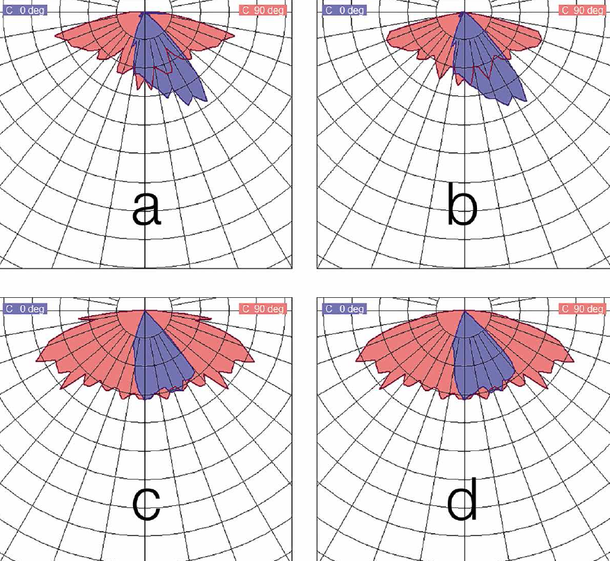
Figure 3 shows the result for two given desired intensity distribution using the specified system introduced in table 4.

Figure 3: The desired light intensity distributions for a target application: DD (top-left) and DW (top-right) and the restored distributions of the separation (bottom row)

Conclusions

It was shown in this paper that in many cases, having a stationary light intensity distribution over the lifetime of an outdoor roadway lighting luminaire, may result in poor uniformity of luminance (both overall- and longitudinal uniformity) by certain environmental conditions, based on the calculations of European Standard EN 13201. In some cases, the distortion of the luminance distribution perceived by a standard observer may even cause disability glare.

Therefore a method was described, that provides controllability of the intensity distribution in order to satisfy lighting requirements with changing optical properties of the environment, thus providing better perceptibility of obstructions, reducing glare and elevating safety for all roadway users. The introduced algorithm aims aligned lumen depreciation of the channels of specifically generated arbitrary intensity distributions that are designed to support the special requirements demanded by this separation.

References:
[1] Lighting for driving, Peter R. Boyce, CRC Press, 2008, ISBN-13:978-0-849-8529-2

[2] The outdoor lighting guide, The Institution of Lighting Engineers, Taylor & Francis, 2005, ISBN 978-0-4153-7007-3

[3] European Standard EN 13201-3 Road lighting - Part 3: Calculation of performance

[4] A genetic algorithm tutorial, Darrell Whitley, Statistics and Computing, 65-85, 1994