Thermal Management of an LED Light Source for Microscopes

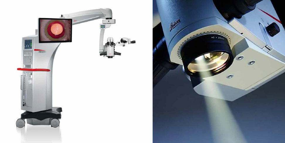
Leica Microsystems develops and manufactures microscopes and scientific instruments for the analysis of microstructures and nanostructures, and is one of the market leaders in microscopy. They are, for instance, renowned for their compound and stereo-microscopes. While being widely recognized for optical precision and innovative technology, they had a major issue with their newly developed light source for the Ophthalmic Microscope.

About Ophthalmic Microscopy

A stable red reflex is one of the most important features of an ophthalmic surgical microscope for cataract surgery. It’s the red reflex that makes the structure of the lens visible and thus makes for an uncompromised view for successful and secure surgery. However, conventional red reflex illumination often decreases during the critical phases of the procedure, such as during phacoemulsification. A new illumination technology based on a high efficient LED Module with four individual beam paths overcomes these drawbacks. This ophthalmic microscope is the first system to feature the new technology. The CoAx4 Illumination provides a stable and consistent red reflex throughout the entire surgical procedure. Both main surgeon and assistant share the same view and full red reflex.

In the initial phase the thermal conditions and the light intensity output in full operation did not meet the specifications of the developers. Through the use of this customized high resolution thermal simulation tool, which was developed at the Institute of Sensor and Actuator Systems of the Vienna University of Technology [1, 2], a promising solution was quickly found. Functional samples were developed; light values were measured, discussed and further optimized. In the course of the optimization, the back-end cooling system with passive heat pipes was also conceived and produced.

About the Thermal Simulation Tool

The simulation tool can solve the stationary and dynamic heat equation. The finite difference method is used as a solution method. At the beginning of the numerical calculation is a choice of the grid and the spatial discretization of the thermal model. Thereupon, the establishment of approximation equations for the spatial calculation area takes place with consideration of the boundary conditions. In the case of transient calculations, initial conditions are taken into account and approximation equations are set up for each time step (temporal discretization). Through this spatial and temporal discretization, the heat conduction equation in differential form is transformed into an algebraic equation system and this is solved with iterative methods.

Heat equation
The heat equation is the basic partial differential equation for describing the temperature field in a stationary medium:

With the temperature T in K of the time t in s the density ρ in kg/m3, the specific heat capacity c in J/kgK, the specific thermal conductivity λ in W/mK and the released internal Heat pi in W/m3.

Finite difference method
By the discretization an orthogonal grid is placed over the model space. In a three-dimensional case, each node has a maximum of six neighbors. If the general case the distances between the grid points along the coordinate axes are arbitrarily selected, this is referred to as a non-uniform grid. The finite difference method is based on the differential form of conservation equations. The differential equations are approximated at each node by replacing the partial derivatives with the difference quotients between the function values at the node points.

Efficient Model Generation

One of the most striking advantages of this simulation tool is the possibility to generate models that are realistic, often built up of complex structures, quickly and flexibly. For discretization, an orthogonal grid is used, which can also be non-equidistant. This divides the model space into cubical volume elements whose size can be adapted to the desired accuracy. A material can be assigned to each of these volume elements, which is represented by a color in the model representation.

The geometry of the tasks occurring in electronics can usually be divided into planar layers. An example of this would be a multilayer circuit board in which insulation layers and copper layers (with the respective conductor pattern) alternate. A complex geometry is usually only present in the lateral extent of these layers. This situation is exploited during model generation. The model space is subdivided into layers of different thickness and each of these layers is filled with colors by means of drawing commands, as known from pixel-oriented drawing programs, whereby the respective material data sets are assigned. Each pixel corresponds to a volume element, the temperature of which is determined by the equation solver (hereinafter referred to as solver). The structures of the individual layers can be taken over from existing drawings, which can be loaded as overlays. In this way complex geometries can also be reproduced very quickly (Figure 2). From the solver, the individual layers are then combined into a real three-dimensional model.

Figure 2: Main window with a model layer each color of the drawn geometry corresponds to a material

Nonlinear solver
The solver used also works with non-linear system of equations, i.e. all material parameters, internal heat and boundary conditions can be taken into account as temperature-dependent variables. In addition, it is possible to specify anisotropic thermal conductivities (e.g. composite materials such as FR4: in the glass fiber direction higher thermal conductivity than perpendicular thereto). The temperature-dependent thermal conductivity is either entered as a polynomial or as a table. Figure 3 shows the input window for determining the temperature-dependent thermal conductivity.

Figure 3: Representation of anisotropic non-linear thermal conductivity in the simulation

Stationary & dynamic solver
The simulation tool allows both stationary and dynamic problems to be solved. In addition to the temperature dependence of the material parameters and internal heat, dynamic dependencies can also be considered. The solvers used allow the solving of equation systems with several 106 unknowns.

Stationary solver
From the general heat equation from Eq (1) is obtained for the case

∂T : ∂t = 0

The stationary heat equation:

The solution of the nonlinear heat equation is achieved in two steps: First, the system of equations is iteratively linearized using the following method: Considering an expression of the form αt with α = at (a is a constant), a non-linearity of the form is produced.

αT = a Ti Ti .

In the iterative method, the past value (time or iterative) is improved by new solutions until the following convergence criterion:

Where n denotes the iteration index. In a second step, the linearized equation system is solved using the iterative SOR method (Successive Over Relaxation).

Dynamic solver
An ADI method (Alternating Direction Implicit) is used to solve the transient heat equation. On the one hand ADI methods can be understood as an iterative method for solving systems of stationary equations. On the other hand, they can be considered as independent method for solving unfixed problems. The main advantage of the ADI methods is the fact that only computation of comparatively small tridiagonal matrices is required, which is numerically favorable.

The class of ADI methods includes a variety of schemes which differ from one another in terms of consistency, stability and convergence. The used Douglas Rachford method is an optimized variant of fully implicit methods and has an accuracy of first order in terms of time. Numerous numerical methods are fast but show strong dependence of the convergence behavior on the selected numerical values and the number of equations of the system (model complexity). The advantage of the modified Douglas Rachford method is the unconditional stability at optimized convergence speed.

Boundary conditions
The flexible and correct choice of the boundary conditions is of great importance for the simulation. A boundary condition for all cells on the model surface needs to be assigned. The simulation allows the definition of a specific boundary condition for each direction of a cell wall (whether a cell wall belongs to the model surface and thus the defined boundary condition must be taken into account in the calculation). Direct input of the following user-definable boundary conditions is possible: constant temperature (Dirichlet boundary condition), constant heat flow (Neumann boundary condition) and heat transfer by radiation and natural convection by input of a temperature - dependent heat transfer coefficient and the input of a material-specific, wavelength-independent emissivity of the surfaces. In addition to the user-defined input of the generally temperature-dependent boundary conditions, it is also possible to use heat radiation and free convection as a program-defined boundary condition. The temperature-dependent heat transfer coefficients of the free convection are then determined taking into account the model geometry of the program itself.

Output module
The simulation results are evaluated in an output module in which the temperature distribution within a model plane is shown in an individually selectable false color display. Figure 4 shows this output module.

Figure 4: Representation of anisotropic non-linear thermal conductivity in the simulation

In addition, it is possible to output temperature profiles in x, y and z directions in diagram form. Figure 5 shows such a temperature profile.

Figure 5: Illustration of a temperature profile

Production and Conclusions

On a copper IMS (Insulated Metal Substrate) with a thermal conductivity of 7.5 W/mK, three high power LEDs are arranged very tightly (Figure 6). The spacing was determined by the optical beam path. The total electrical power of the LED module is 27 W. The hot spot is the middle LED, which was assembled in Chip on Board (COB) technology to meet the very narrow space requirement. Both outer LEDs are mounted with conventional Surface Mount Technology (SMT). The middle LED is operated with 8 W. This means about 6 W power loss must be dissipated thermally between the two hot LEDs. This could only be realized by means of suitable copper structures on the IMS that have been simulated and optimized. The IMS is soldered on the cooling block. This metal interconnection was important for the thermal management and to assure that no oxidation of the interface or change of the thermal resistance occurs over the lifetime. The IMS design performance proved to be so good that the light source can be operated with 125% power without the LEDs reaching the maximum permissible junction temperature. The heat is transported from the copper block via two heat pipes to the cooling fins (Figure 7). This evaporation and condensation process in the heat pipe works in the range of the velocity of sound. The heat pipes are soldered to the copper block to ensure consistent performance over the lifetime. A "Burn in" for all modules during which the thermal transitions are measured and documented before delivery ensures that all production units have the same quality.

Figure 6: LED module soldered to cooling block

With extraordinary good thermal management it is even possible to drive LEDs harder than originally foreseen to satisfy the special demands of an application. Just innovative product design based on sophisticated simulation tools in combination with the correct material selection, excellent manufacturing methods and manufacturing capabilities lead to superior results.

Figure 7: Assembly of heat pipes in the clean room

References:
[1] Hanreich, G., Nicolics, J., Musiejovsky, L., “High resolution thermal simulation of electronic components,” Microelectronics Reliability, Vol. 40 (2000), pp. 2069-2076.

[2] Nicolics, J., “TRESCOM”, White Paper, Institute of Sensor and Acutator Systems, Vienne University of Technology, 2008