Variability in LED Production and the Impact on Performance
LEDs are subject to manufacturing deviations, which have an impact on the end product. Benoit Bataillou and T. Merelle, guest authors from Pi Lighting, review the surprisingly large impact on LED performance and light quality. They used traditional as well as modern indicators like CRI and TM-30 as well as the latest circadian indices to measure. The results are explained by spectral modeling and a variability study. They show the large impact on CRI, even with small deviations inside the same bin.
One of the most known but least understood subjects is LED variability. Variability is, as Wikipedia defines it, how a distribution or series of data is stretched or squeezed. – But where does it come from?
A white LED is a little system. A semiconductor device (or several devices), is covered with an encapsulant and phosphorus connected inside a package, sometimes with an extra primary optics on top. For those who come from the “Silicon world”, the first striking difference in the LED world is the material defects quantities- Without going in too many details, one can assume about 5 to 7 orders of magnitude between the density of crystalline defects within the grown LED material and a regular epiwafer for the silicon world [1].
The structure itself, the emissive part of the blue die, is a stack of layers of different composition, each of them of an average 2 to 3 nanometers thick [2]. This is a crystalline layer of 6 atoms thick, covering the area of the device (typically 0.5 to 1 square millimeter). In this structure called quantum wells, each variation of thickness leads to a different light emission. There is a batch effect (lot to lot), a tooling effect (tool to tool) and statistical effects (variation of well thicknesses).

Figure 1: Royal blue InGaN LED, also nicknamed a “pump”
Contributors to Variations
So first, the light emission of blue has intrinsically a large variability, and those large peaks a blue LED shows are well known. Showing those peaks to experts in II-VI semiconductors or GaAs epitaxy engineers, I overheard in the lab that those peaks were more “potatoes” than peaks. The position of the peak also moves with the content of the quantum wells and their average thickness.
Second, the rest of the LED also brings in variability. Phosphorus is a mix of several compounds, doped garnets embedded in a matrix. This material has the property to absorb (not equally) a set of wavelengths and convert them
(not equally) to longer wavelengths.
Third, the package and reflections within the package cause another source of variability, slight misalignment of the die within the package can cause different light paths, and such different color shifts.
The result of this, and everything above depending on current and temperature, is white light that the eye (which is quite a nice color sensitive device) detects.
From this over-summarized view, LED production can be expected to be a fine cuisine (and cuisine is an art where I come from), and will show consequent variability in the resulting color points.
What does it give us? A population of “identical” LEDs, which are actually far from identical, from which the manufacturer will select bins (color bins, Vf bins, CRI bins, etc.), to reduce variability. In the rest of the paper ANSI binning will be used as basis, as it’s the most popular binning approach. But all apply to divide the color space.
, and the model fit (blue)") Figure 2: The champion white LED spectrum(orange), and the model fit (blue)
Figure 2: The champion white LED spectrum(orange), and the model fit (blue)
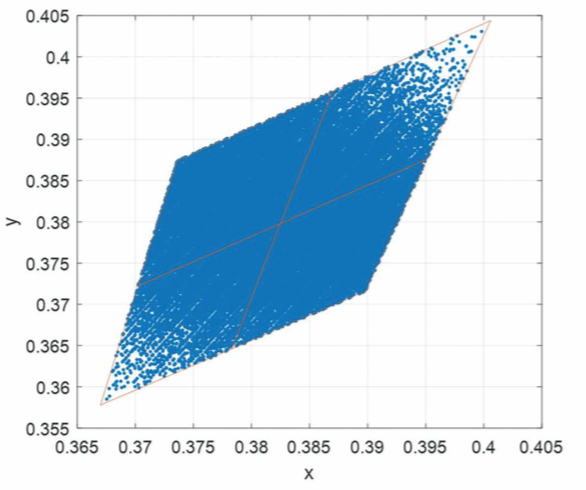
 Figure 3: 4000 K ANSI bin LED divided into 4 sub- bins, and 85000 color points of virtual LEDs obtained by modifying the champion white LED
Simulating Variability
The following example of simulation of variability demonstrates a simple case. Starting from measuring a single LED, from a manufacturer that was nice enough to participate in this study, a model was developed to fit it.
Starting from this “champion LED”, the spectrum will slightly be modified to evaluate the consequences.
Being relatively satisfied with the fit quality, the two peaks (the blue peak and “yellow” peak) were extracted. Then, the position of the blue peak was slightly changed, and the resulting variations in the phosphorus composition were simulated by changing the height of the yellow peak.
A “virtual binning”, will be done and the spectra chosen with color points staying inside the four “ANSI 4000 K” bins [3].
Of course, models must be validated. To do a quick check, two extra LEDs were measured, provided by the same manufacturer, located in different sub-bins of the same large bin (we are trying to obtain color points far away from the champion LED color point).
Those LEDs were measured looking in the large color cloud
for two color points as close as possible. Then the spectra between the original simulation and a real LED located at same color point were compared. The result is shown in figures 4.
 Figures 4: Two new LEDs, measured and compared with spectra in cloud above where the color point is as close as possible
From the figures above can be recognized that there are some slight differences, so the validation of the model is not perfect, but overall the spectrum is well represented.
Now what? Assuming that a population of LEDs is adequately correct simulated, it is possible to have a look at the variability of the different colorimetry metrics.
Logically, CCT varies of 225 K (the size of the bin). More interesting is the variation of CRI within this color cloud.
There is a variation range of approximately 6 points of CRI,
and 29 points of R9. In terms of percentages, R9 has variability close to 300% (3 standard deviations), ranging from negative values up to 25.
It is noteworthy to mention that the only cause of this variation is the small spectral changes from an LED to another within the same bin.
Circadian Indexes and MR Variability CS
Circadian index CS and MR (Melanopic ratio) represent the disturbance of the circadian clock by a given light. Circadian index follow a rather complex formula. Details of the calculations can be found in the publications from Lighting Research Center/RPI [4].
The CL is the complex basic A formula needed to calculate CS, which is then calculated as using the CLA [5], shown in figures 5a&b.
 due to the small spectral differences within ANSI 4000 K bin") Figure 5: CRI and R9 variations (and normal fits) due to the small spectral differences within ANSI 4000 K bin
Figure 5: CRI and R9 variations (and normal fits) due to the small spectral differences within ANSI 4000 K bin
This metric is spectral AND illumination dependent, so the calculations are done at 250 lux. Looking at the cloud of LEDs, one will recognize a surprisingly large CS distribution within the 4000 K bin.
CS average is 0.17, with a variation (3 standard deviations) of 28%.
 and CS (b)") Figures 6a&b: Equations to calculate CLA (a) and CS (b)
Figures 6a&b: Equations to calculate CLA (a) and CS (b)
 Figure 7: CS@250lux distribution within 4000K ANSI bin
 Figure 8: MR calculation - the Melanopic curve above, times a spectrum, divided by flux, is the MR
MR
MR or Melanopic Ratio represents the quantity of light present under a specific curve (similar to the Mc quantity in the CLA/CS equation), divided by the luminous flux. This gives a “circadian content” which is convenient to use practically. This quantity is only spectral dependent. The MR times the illumination gives the EML, Equivalent Melanopic Lux.
Applying this to the population of 4000 K LEDs, one will see that the distribution centered at MR=0.61 ±14% (3 standard deviations).
Conclusions
The investigation and simulation showed that within a single ANSI bin, the variability created a surprisingly large spread on all studied quantities. The CRI, R9, Cs, MR, had variations between 14% and 300%, for a single ANSI bin.
Going further, it can be seen that the specifications are intricate. The CRI specification a manufacturer will provide, or a user will ask of a manufacturer, is dependent on the provide or accept color spread.
The more and more popular circadian metrics will also depend on the other specifications.
As for the color cloud itself; conclusions on the impact of variability can be made by comparing two different spectra that look “similar” and their color shifts.
The color points of those two spectra, which look “similar”, are not in the same color bin. They are at 0.009 u’v’ distance, which is what is often assume to be about 9 SDCM or 9 MacAdam ellipses. They also have a difference of 283K and a difference in R9 of 150%. In practical use, one would consider those two LEDs to be very different one from each other, despite a very similar spectrum.
Color points, which are a simulation of how the human color perception works, are very sensitive to any spectral variation. This means LED users must be careful when specifying too narrowly.
And on the LED manufacturer side, offering very narrow color spreads is also a natural tendency, but variability can lead to large yield losses and unrealistic expectations from customers.
Finally, the model can be extended to individual phosphorus peaks, linked to more “physical” parameters (phosphorus thicknesses and content, etc.), as a basis for a more detailed study.
 Figure 9: Two “similar” spectra picked in the color cloud. Same blue pump, <5% difference in W/nm
References:
[1] Shih, H.-Y. e. (s.d.). Ultralow threading dislocation density in GaN epilayer on near-strain-free GaN compliant buffer layer and its applications in hetero-epitaxial LEDs. Sci. Rep. 5, 13671;
[2] http://www.sees.cinvestav.mx/download/20-2015.pdf
[3] https://www.energystar.gov/ia/partners/product_specs/program_reqs/SSL_prog_req.pdf?d519-671a
[4] LRC: MS Rea & al, Modelling the spectral sensitivity of the human circadian system, Lighting Res. Technol. 2011; 0: 1–12
[5] Circadian Light, Rea et al. Journal of Circadian Rhythms 2010, 8:2
(c) Luger Research e.U. - 2017
